Machine Learning Basics–Regression Analysis–Part 1

 

Data is all around us, its happening, At the simplest form data is a set of variables (of course with values). While working on a database on any domain , once we have a relatively  okay understanding of the entities and we start to look for relationships within the entity or the variable. We do stumble upon and have a gut feeling which tells a variable y is dependent on a variable x OR a set of variables (x1,,x2…xn).

To a certain degree we can predict the new value of y based on x. We see there is a clear relationship between y and x.  The process of estimating relationships among variables is termed as Regression Analysis.  Here the focus is between  a dependent variable and one of more independent variables ( called the predictors).

 

There are various types of Regression Analysis example Linear, Logistic, Polynomial….  each of them are used for a specific purpose.

Regression Analysis requires a prior knowledge on the dataset and in order to estimate the forecasted value of the dependent variable. There is a need of having a dataset with defined outcomes of the dependent variable which will be used to train the algorithm.  Regression set of algorithm are a part of supervised learning.

 

Different Type of Regression

Linear Regression – The relationship between the dependent and independent variables is such that the nature of the regression  line is linear.

Linear Regression establishes a relationship between dependent variable (Y) and one or more independent variables (X) using a best fit straight line (also known as regression line).The  best fit straight line is generally achieved with Least Square Method. It is most commonly used for fitting a regression line. It calculates the best fit line for the observed data by minimizing the sum of squares  of the vertical deviations from each data points to the line.

Example on Linear Regressions.

As an example for Linear Regression we are taking the

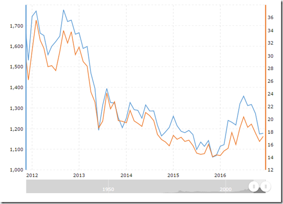
Gold and Silver Price Correlation

The basic plot of the same can be seen below. The data and code for the same can be found here. The data consists of last 1 year data, If one needs the complete data for last 10 years you can download the same from many of the free data sources or refer to http://www.macrotrends.net/2517/gold-prices-vs-silver-prices-historical-chart.

For trying out linear regression the code is pretty straightforward

install.packages("Quandl")
library(Quandl)
install.packages("devtools")
library(devtools)
install_github("quandl/quandl-r")

goldprices =  Quandl("LBMA/GOLD")
silverprices = Quandl("LBMA/SILVER")

goldpricesshortterm = goldprices[1:730,]
silverpricesshortterm = silverprices[1:730,]

shtsilver = data.frame(silverpricesshortterm,goldpricesshortterm)
sfit = lm(shtsilver$USD..AM.~shtsilver$USD)
summary(sfit)

Used Quandl for gold and silver price data.  Have applied Linear Regression Model to last 2 years of data.

 

Interpreting the results of lm

The summary of the lm result what we look for

1. Residuals are essentially the difference between the actual observed response , We look for a symmetrical distribution across these points on the mean value zero (0). In this case we see a symmetrical distribution

2. The t-statistic values are relatively far away from zero and are large relative to the standard error, which could indicate a relationship exists. In general, t-values are also used to compute p-values

3.In our example, the RSquared we get is 0.8028. Or roughly 80% of the variance found in the response variable (gold prices) can be explained by the predictor variable (silver price)